When seeking to build a machine learning model, data is the food you add to a cooking pot, and Scaling is the final spice and salt that completes the meal: the model.

Introduction

Data comes in various formats, representing different variables. In this nature, the data is not on a similar scale and would not lead to the optimal model we want to build. Besides, when features have different ranges, algorithms can be biased towards higher values, leading to suboptimal models. Machine Learning algorithms often assume that input features lie on a similar scale. Scaling ensures that each feature contributes approximately proportionately to the final prediction.

Understanding the Need for Scaling

Assume you want to predict whether someone will buy a house in the next 12 months. The dataset includes features like Age, ranging from 20 to 40, and Annual Income, ranging from 10,000 to 150,000. Without scaling, a machine learning model may incorrectly learn that Annual Income is more important than Age simply because of the larger numerical values, potentially leading to suboptimal predictions.

Feature Scaling: The Process

It is a process that involves transforming the features of your dataset so that they share a common scale. This is critical before fitting the model, especially for algorithms sensitive to feature magnitude, such as gradient-boosted trees and logistic regression. Chip Huyen describes feature scaling as one of the simplest things you can do to improve your model's performance. Neglecting this vital step would lead to not-so-good predictions from your model.

There are various techniques for scaling your features to improve your model.

• Standardization

• Min-Max Scaling

• Robust Scaling

1. Standardization (Z-score Normalization)

Standardization transforms your data such that the resultant distribution has a mean of 0 and a standard deviation of 1. The formula for standardization is:

$$z = \frac{x - \mu}{\sigma}$$

Where:

• z is the standardized value.

• x is the original value.

• μ is the mean of the feature values.

• σ is the standard deviation of the feature values.

It is useful for algorithms that assume your data is normally distributed, like Support Vector Machines.

from sklearn.preprocessing import StandardScaler
scaler = StandardScaler()
age_standardized = scaler.fit_transform(data[['Age']])

1. Min-Max Scaling

Min-Max Scaling shrinks the range of the data within a specified range, often between 0 and 1. The formula for Min-Max Scaling is:

$$X_{\text{scaled}} = \frac{X - X_{\text{min}}}{X_{\text{max}} - X_{\text{min}}}$$

Where:

• Xscaled​ is the scaled value.

• X is the original value.

• Xmin​ is the minimum value of the feature.

• Xmax​ is the maximum value of the feature.

It is a scaling technique beneficial for algorithms sensitive to small variations, like Neural Networks. A simple code for implementation is shown below:

from sklearn.preprocessing import MinMaxScaler
scaler = MinMaxScaler()
age_minmax = scaler.fit_transform(data[['Age']])

1. Robust Scaling

Robust Scaling uses the median and the interquartile range (IQR), making it less sensitive to outliers. The formula for Robust Scaling is:

$$X_{\text{robust}} = \frac{X - Q_1}{Q_3 - Q_1}$$

Where:

• Xrobust​ is the robust scaled value.

• X is the original value.

• Q1​ is the first quartile (25th percentile) of the feature values.

• Q3​ is the third quartile (75th percentile) of the feature values.

It is a better choice for datasets where outliers might otherwise distort the scaled values.

from sklearn.preprocessing import RobustScaler
scaler = RobustScaler()
age_robust = scaler.fit_transform(data[['Age']])

Implementation

For the example stated earlier, we are going to use this data:

data = pd.DataFrame({
    'Age': [27, 27, 40, 35, 33, 20],
    'Annual Income': [50000, 100000, 150000, 50000, 60000, 10000]
})

We then proceed to scale the data using the different techniques as shown below:

# StandardScaler
standard_scaler = StandardScaler()
data['Age_Standardized'] = standard_scaler.fit_transform(data[['Age']])
data['Income_Standardized'] = standard_scaler.fit_transform(data[['Annual Income']])

# MinMaxScaler
minmax_scaler = MinMaxScaler()
data['Age_MinMax'] = minmax_scaler.fit_transform(data[['Age']])
data['Income_MinMax'] = minmax_scaler.fit_transform(data[['Annual Income']])

# RobustScaler
robust_scaler = RobustScaler()
data['Age_Robust'] = robust_scaler.fit_transform(data[['Age']])
data['Income_Robust'] = robust_scaler.fit_transform(data[['Annual Income']])

Lastly, we visualize the effect of these scaling techniques.

import matplotlib.pyplot as plt

# Plotting histograms for the scaled and unscaled data
def plot_histograms(data):
    fig, axs = plt.subplots(2, 4, figsize=(24, 10))

    # Original Data
    axs[0, 0].hist(data['Age'], bins=10, alpha=0.7, color='blue')
    axs[0, 0].set_title('Original Age Data')
    axs[1, 0].hist(data['Annual Income'], bins=10, alpha=0.7, color='blue')
    axs[1, 0].set_title('Original Annual Income Data')

    # Standardized Data
    axs[0, 1].hist(data['Age_Standardized'], bins=10, alpha=0.7, color='orange')
    axs[0, 1].set_title('Standardized Age Data')
    axs[1, 1].hist(data['Income_Standardized'], bins=10, alpha=0.7, color='orange')
    axs[1, 1].set_title('Standardized Annual Income Data')

    # Min-Max Data
    axs[0, 2].hist(data['Age_MinMax'], bins=10, alpha=0.7, color='green')
    axs[0, 2].set_title('Min-Max Age Data')
    axs[1, 2].hist(data['Income_MinMax'], bins=10, alpha=0.7, color='green')
    axs[1, 2].set_title('Min-Max Annual Income Data')

    # Robust Data
    axs[0, 3].hist(data['Age_Robust'], bins=10, alpha=0.7, color='red')
    axs[0, 3].set_title('Robust Age Data')
    axs[1, 3].hist(data['Income_Robust'], bins=10, alpha=0.7, color='red')
    axs[1, 3].set_title('Robust Annual Income Data')

    for ax in axs.flat:
        ax.set(xlabel='Value', ylabel='Frequency')

    # Hide x labels and tick labels for top plots and y ticks for right plots.
    for ax in axs.flat:
        ax.label_outer()

    plt.tight_layout()
    plt.show()

plot_histograms(data)

The result is shown below.

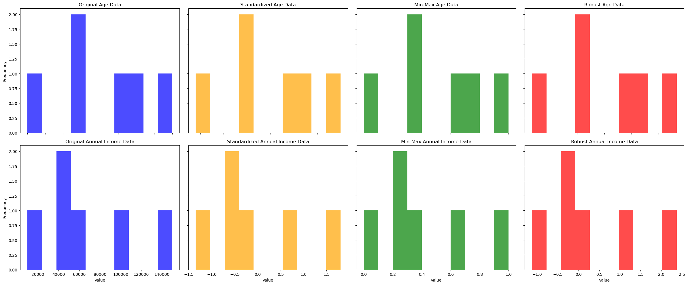
From the result of the scaled data, we can see that both variables were brought to a similar scale, thus making it possible to build a model that would not decriminalize the features.

Conclusion

Selecting the correct scaling technique can dramatically improve your model's performance. It is also possible to decide which scaling method to implement by understanding the distribution and nature of your data and the requirements of the machine-learning algorithms you plan to use. The histograms provide a visual affirmation of how each technique affects the data, offering insights into the transformation process and ensuring a more balanced representation of features within your model.

References

Huyen, C. (2022). Designing Machine Learning Systems (1st ed.). O’Reilly Media, Inc. [oreilly.com/library/view/designing-machine-..

Thank you for your time!